In this notebook I will attempt to cluster eCommerce item data by their names. The data is from an outdoor apparel brand’s catalog. I want to use the item names to find similar items and group them together. For example, if it’s a t-shirt it should belong in the t-shirt group.
The steps to accomplish this goal will be:
- Cleaning the data to just include the name (pandas)
- Transform the corpus into vector space using tf-idf (Sci Kit)
- Calculating cosine distance between each document as a measure of similarity (Sci Kit)
- Hierarchical Clustering and Dendrogram (Scipy)
- Cluster the documents with k-means (Sci Kit)
- Use MDS to reduce the dimension
- Plot the clusters (matplotlib)
The dataset consists of 500 actual SKUs from an outdoor apparel brand’s product catalog downloaded from Kaggle (https://www.kaggle.com/cclark/product-item-data).
I used http://brandonrose.org/clustering as a reference for this project. He has a lot of interesting projects with great explanations in his blog.
Cleaning Data
Import the packages needed
import os
import pandas as pd
import re
import numpy as np
Read the data.
df = pd.read_csv('sample-data.csv')
A quick look at the data. There are 2 columns, id and description.
df.head()
| id | description | |
|---|---|---|
| 0 | 1 | Active classic boxers - There's a reason why o... |
| 1 | 2 | Active sport boxer briefs - Skinning up Glory ... |
| 2 | 3 | Active sport briefs - These superbreathable no... |
| 3 | 4 | Alpine guide pants - Skin in, climb ice, switc... |
| 4 | 5 | Alpine wind jkt - On high ridges, steep ice an... |
Let’s take a closer look at the description and what it has. It starts off with the name then a long description then ending with material detail. I am only interested in the name for this project so I will separate it out.
print df['description'][5]
Ascensionist jkt - Our most technical soft shell for full-on mountain pursuits strikes the alpinist's balance between protection and minimalism. The dense 2-way-stretch polyester double weave, with stitchless seams, has exceptional water- and wind-resistance, a rapid dry time and superb breathability. Pared-down detailing provides everything you need and nothing more: a 3-way-adjustable, helmet-compatible hood; a reverse-coil center-front zipper with a DWR (durable water repellent) finish; large external handwarmer pockets (with zipper garages) that are placed above the harness-line; an internal security pocket; articulated arms; self-fabic cuff tabs; a drawcord hem. Recyclable through the Common Threads Recycling Program.<br><br><b>Details:</b><ul> <li>"Dense stretchy polyester double-weave fabric is exceptionally water- and wind-resistant and is spandex-free for fast dry times; Stitch-free, lap-glued seams speed dry time, improve water resistance and decrease bulk"</li> <li>"Helmet-compatible, 3-way-adjustable hood; brushed chamois patches for chin and neck comfort"</li> <li>DWR-(durable water repellent) finished center-front zipper; external pockets: two handwarmers fit skins and have zipper garages and DWR finish on zippers</li> <li>Internal security pocket</li> <li>Articulated arms</li> <li>"Low-profile, laminated, self-fabric cuff tabs"</li> <li>Drawcord hem</li></ul><br><br><b>Fabric: </b>5.3-oz 100% polyester (45% recycled) double weave with 2-way-stretch and Deluge DWR finish. Recyclable through the Common Threads Recycling Program<br><br><b>Weight: </b>(553 g 19.2 oz)<br><br>Made in China.
This function splits the description returning only the name.
def split_description(string):
    # name
    string_split = string.split(' - ',1)
    name = string_split[0]

    return name
Let’s put the clean data into a new data frame.
df_new = pd.DataFrame()
df_new['name'] = df.loc[:,'description'].apply(lambda x: split_description(x))
df_new['id'] = df['id']
This function removes numbers and extra spaces from the name.
def remove(name):
    new_name = re.sub("[0-9]", '', name)
    new_name = ' '.join(new_name.split())
    return new_name
Let’s apply the function above.
df_new['name'] = df_new.loc[:,'name'].apply(lambda x: remove(x))
Now the data is all nice and clean.
df_new.head()
| name | id | |
|---|---|---|
| 0 | Active classic boxers | 1 |
| 1 | Active sport boxer briefs | 2 |
| 2 | Active sport briefs | 3 |
| 3 | Alpine guide pants | 4 |
| 4 | Alpine wind jkt | 5 |
TF-IDF
Import TF-IDF vectorizer from sklearn.
from sklearn.feature_extraction.text import TfidfVectorizer
Let’s set up the parameters for our TF-IDF vectorizer.
I want to use the inverse document frequency so I set it as True.
By setting stop words as english it will remove irrevelant words such as to, and, etc.
The ngram range splits our documents in 1 term, 2 terms, … 4 terms.
Min df is used for removing terms that appear too infrequently, 0.05 means ignore terms that appear less than 1% of the documents. Max df is vice versa, ignore terms that appear more than 90% of the documents.
tfidf_vectorizer = TfidfVectorizer(
                                   use_idf=True,
                                   stop_words = 'english',
                                   ngram_range=(1,4), min_df = 0.01, max_df = 0.8)
Now that the vectorizer is set I will fit and transform the data.
%time tfidf_matrix = tfidf_vectorizer.fit_transform(df_new['name'])
CPU times: user 10.5 ms, sys: 2.29 ms, total: 12.8 ms
Wall time: 13 ms
The parameters have narrowed down to 85 important terms in the matrix.
print(tfidf_matrix.shape)
print tfidf_vectorizer.get_feature_names()
(500, 85)
[u'active', u'baby', u'baggies', u'baggies shorts', u'belt', u'board', u'board shorts', u'borderless', u'bottoms', u'briefs', u'btm', u'cap', u'cap bottoms', u'cap crew', u'cap zip', u'cap zip neck', u'capris', u'cargo', u'continental', u'cotton', u'crew', u'ctn', u'ctn jeans', u'dress', u'fit', u'fit organic', u'fit organic ctn', u'fit organic ctn jeans', u'girl', u'glory', u'graphic', u'guide', u'guide pants', u'guidewater', u'hat', u'hemp', u'hoody', u'island', u'jeans', u'jkt', u'live', u'live simply', u'logo', u'logo shirt', u'lw', u'lw travel', u'merino', u'morning', u'morning glory', u'neck', u'organic', u'organic ctn', u'organic ctn jeans', u'pack', u'pants', u'polo', u'poster', u'print', u'rain', u'rain shadow', u'rashguard', u'runshade', u'shadow', u'shirt', u'shorts', u'simply', u'skirt', u'socks', u'solid', u'stretch', u'sun', u'sweater', u'synch', u'tank', u'tee', u'torrentshell', u'trails', u'travel', u'vest', u'vitaliti', u'waders', u'watermaster', u'zip', u'zip jkt', u'zip neck']
I calculate the cosine similarity between each document. By subtracting 1 will provide the cosine distance for plotting on a 2 dimensional plane.
from sklearn.metrics.pairwise import cosine_similarity
dist = 1.0 - cosine_similarity(tfidf_matrix)
print dist
[[  0.00000000e+00   3.25246908e-01   3.25246908e-01 ...,   1.00000000e+00
    1.00000000e+00   1.00000000e+00]
 [  3.25246908e-01  -2.22044605e-16  -2.22044605e-16 ...,   1.00000000e+00
    1.00000000e+00   1.00000000e+00]
 [  3.25246908e-01  -2.22044605e-16  -2.22044605e-16 ...,   1.00000000e+00
    1.00000000e+00   1.00000000e+00]
 ...,
 [  1.00000000e+00   1.00000000e+00   1.00000000e+00 ...,   1.00000000e+00
    1.00000000e+00   1.00000000e+00]
 [  1.00000000e+00   1.00000000e+00   1.00000000e+00 ...,   1.00000000e+00
    0.00000000e+00   4.67823979e-01]
 [  1.00000000e+00   1.00000000e+00   1.00000000e+00 ...,   1.00000000e+00
    4.67823979e-01   0.00000000e+00]]
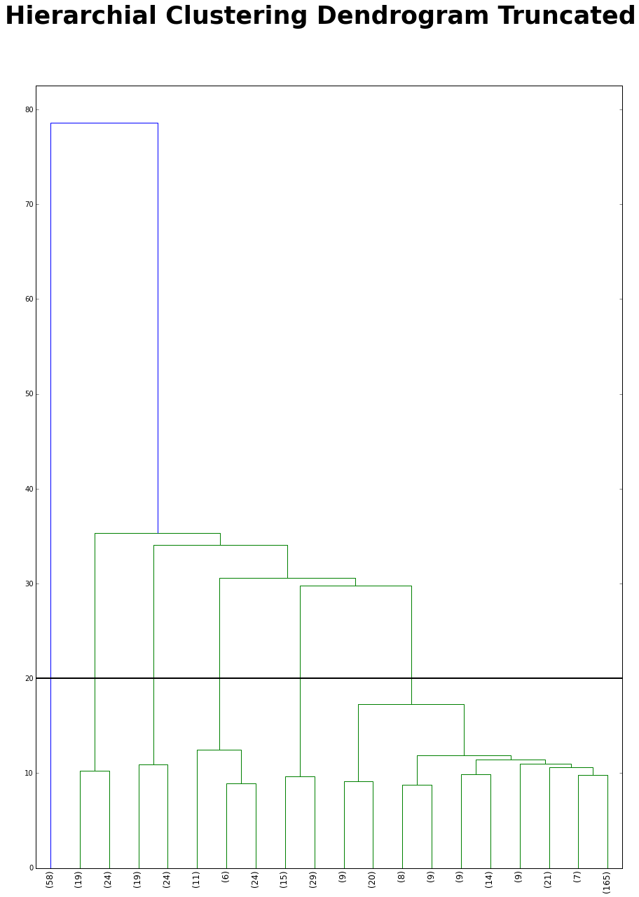
Before I begin the kmeans clustering I want to use a hierarchial clustering to figure how many clusters I should have. I truncated the dendrogram because if I didn’t the dendrogram will be hard to read. I cut at 20 because it has the second biggest distance jump (the first big jump is at 60). After the cut there are 7 clusters.
from scipy.cluster.hierarchy import ward, dendrogram
import matplotlib.pyplot as plt
%matplotlib inline
linkage_matrix = ward(dist) #define the linkage_matrix using ward clustering pre-computed distances

fig, ax = plt.subplots(figsize=(15, 20)) # set size
ax = dendrogram(linkage_matrix,
                truncate_mode='lastp', # show only the last p merged clusters
                p=20, # show only the last p merged clusters
                leaf_rotation=90.,
                leaf_font_size=12.)


plt.axhline(y=20, linewidth = 2, color = 'black')

fig.suptitle("Hierarchial Clustering Dendrogram Truncated", fontsize = 35, fontweight = 'bold')

fig.show()
K-Means Clustering
Let’s fit k-means on the matrix with a range of clusters 1 - 19.
from sklearn.cluster import KMeans
num_clusters = range(1,20)

%time KM = [KMeans(n_clusters=k, random_state = 1).fit(tfidf_matrix) for k in num_clusters]
CPU times: user 2.48 s, sys: 6.22 ms, total: 2.48 s
Wall time: 2.49 s
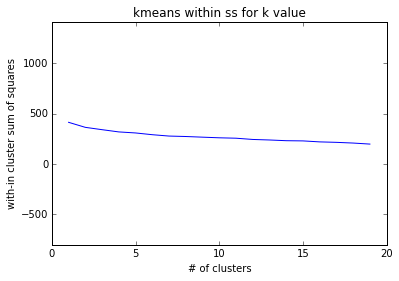
Let’s plot the within cluster sum of squares for each k to see which k I should choose.
The plot shows a steady decline from from 0 to 19. Since the elbow rule does not apply for this I will choose k = 7 because of the previous dendrogram.
import matplotlib.pyplot as plt
%matplotlib inline
with_in_cluster = [KM[k].inertia_ for k in range(0,len(num_clusters))]
plt.plot(num_clusters, with_in_cluster)
plt.ylim(min(with_in_cluster)-1000, max(with_in_cluster)+1000)
plt.ylabel('with-in cluster sum of squares')
plt.xlabel('# of clusters')
plt.title('kmeans within ss for k value')
plt.show()
I add the cluster label to each record in df_new
model = KM[6]
clusters = model.labels_.tolist()
df_new['cluster'] = clusters
Here is the distribution of clusters. Cluster 0 has a records, then cluster 1. Cluster 2 - 4 seem pretty even.
df_new['cluster'].value_counts()
0    244
1     73
2     46
6     45
3     44
5     33
4     15
Name: cluster, dtype: int64
I print the top terms per cluster and the names in the respective cluster.
print("Top terms per cluster:")
print
order_centroids = model.cluster_centers_.argsort()[:, ::-1]
terms = tfidf_vectorizer.get_feature_names()
for i in range(model.n_clusters):
    print "Cluster %d:" % i,
    for ind in order_centroids[i, :10]:
        print ' %s' % terms[ind],
    print
    print "Cluster %d names:" %i,
    for idx in df_new[df_new['cluster'] == i]['name'].sample(n = 10):
        print ' %s' %idx,
    print
    print
Top terms per cluster:

Cluster 0:  vest  dress  print  skirt  active  poster  solid  merino  lw  socks
Cluster 0 names:  Lw everyday socks  Corinne dress  ' logo t-shirt  All-time shell  Baby synch vest  All weather training top  Symmetry w poster  Barely hipster  Hip pack  Down sweater

Cluster 1:  shirt  merino  island  runshade  polo  baby  logo  guidewater  fit organic ctn jeans  ctn jeans
Cluster 1 names:  Merino t-shirt  S/s sol patrol shirt  The more you know t-shirt  Vintage logo pkt t-shirt  S/s el ray shirt  L/s island hopper shirt  Rockpile t-shirt  Squid t-shirt  Sleeveless a/c shirt  Caribou north wind t-shirt

Cluster 2:  pants  guide pants  guide  borderless  cargo  continental  torrentshell  zip  rain shadow  shadow
Cluster 2 names:  Inter-continental pants  Compound cargo pants  Borderless trek pants  Borderless zip-off pants  Lithia pants  Shelled insulator pants  Alpine guide pants  Simple guide pants  Torrentshell pants  Custodian pants

Cluster 3:  shorts  board  board shorts  borderless  baggies shorts  baggies  cargo  continental  trails  guide
Cluster 3 names:  Ultra shorts  Solimar shorts  Inga shorts  Cotton board shorts  Boardie shorts  Borderless shorts- in.  Rock guide shorts  Stand up shorts- in.  Wavefarer board shorts- in.  Compound cargo shorts

Cluster 4:  simply  live  live simply  shirt  organic  girl  baby  tee  polo  tank
Cluster 4 names:  Girl's live simply seal t-shirt  Live simply guitar t-shirt  Baby live simply seal t-shirt  Live simply deer t-shirt  Girl's live simply deer t-shirt  Simply organic tank  Live simply guitar t-shirt  Simply organic top  Simply organic polo  Baby live simply deer t-shirt

Cluster 5:  cap  cap bottoms  bottoms  cap crew  crew  shirt  neck  graphic  cap zip neck  cap zip
Cluster 5 names:  Cap graphic t-shirt  Cap scoop  Cap cap sleeve  Cap bottoms  Cap bottoms  Cap t-shirt  Cap crew  Cap bottoms  Cap t-shirt  Cap bottoms

Cluster 6:  jkt  zip jkt  guide  zip  torrentshell  stretch  sweater  trails  lw  cap
Cluster 6 names:  Guide jkt  Alpine wind jkt  El cap jkt  Deep wading jkt  Baby duality jkt  Storm light jkt  R full-zip jkt  R jkt  Alpine wind jkt  Aravis jkt
I reduce the dist to 2 dimensions with MDS. The dissimilarity is precomputed because we provide 1 - cosine similarity. Then I assign the x and y variables.
import matplotlib.pyplot as plt
import matplotlib as mpl

from sklearn.manifold import MDS

mds = MDS(n_components=2, dissimilarity="precomputed", random_state=1)

pos = mds.fit_transform(dist)

xs, ys = pos[:, 0], pos[:, 1]
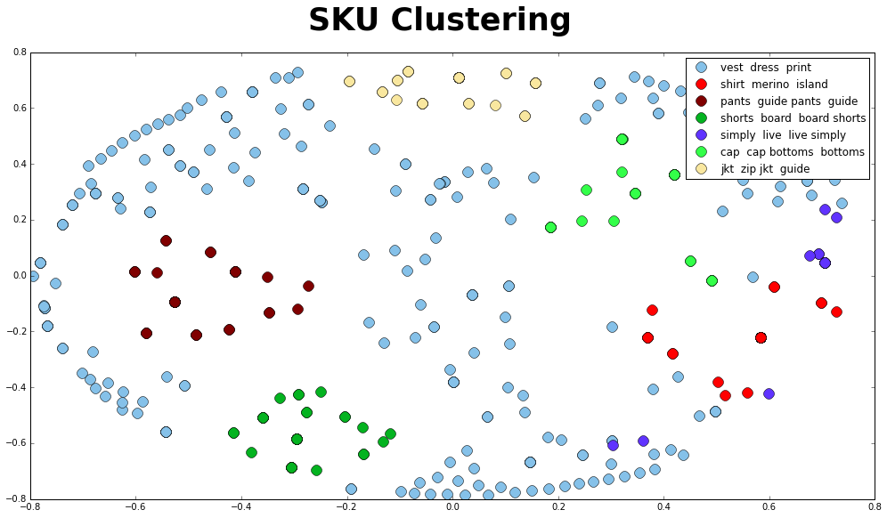
Let’s plot the clusters with colors and name each cluster as the top term so it is easier to view. The clusters look good except maybe cluster 0 “vest dress shirt”. There seems to be some uncertainty. I am not sure what is causing this issue, but I was able to find out that TF-IDF works better on longer text.
cluster_colors = {0: '#85C1E9', 1: '#FF0000', 2: '#800000', 3: '#04B320',
                  4: '#6033FF', 5: '#33FF49', 6: '#F9E79F', 7: '#935116',
                  8: '#9B59B6', 9: '#95A5A6'}
cluster_labels = {0: 'vest  dress  print', 1: 'shirt  merino  island',
                  2: 'pants  guide pants  guide', 3: 'shorts  board  board shorts',
                  4: 'simply  live  live simply', 5: 'cap  cap bottoms  bottoms',
                  6: 'jkt  zip jkt  guide'}

#some ipython magic to show the matplotlib plots inline
%matplotlib inline

#create data frame that has the result of the MDS plus the cluster numbers and titles
df_plot = pd.DataFrame(dict(x=xs, y=ys, label=clusters, name=df_new['name']))

#group by cluster
groups = df_plot.groupby('label')

# set up plot
fig, ax = plt.subplots(figsize=(17, 9)) # set size

for name, group in groups:
    ax.plot(group.x, group.y, marker='o', linestyle='', ms=12,
            label = cluster_labels[name],
            color = cluster_colors[name])
    ax.set_aspect('auto')

ax.legend(numpoints = 1)

fig.suptitle("SKU Clustering", fontsize = 35, fontweight = 'bold')

plt.show()